January 22nd 2026: Building and Running Python Jobs

Recording of the first part of the meeting

Environments and help pages referenced

Python Basics Ubuntu Environment (needs app login)

Machine-generated transcript

Introduction

Let’s get started. Today we will talk about building and running Python jobs on DECTRIS CLOUD. This is a new way of running analysis jobs where you do not have to use Bash scripting if you are not comfortable with that.

The plan for today is to first explain the difference between Python jobs as they are currently implemented and traditional Bash jobs. Then I will show how to build a Python job and what the updated job execution interface looks like, as this has been recently improved.

Building a Python Job Template

I will start by going to app.dectris.cloud. Traditionally, jobs on DECTRIS CLOUD have been created using Bash scripting. I will show an example of how this looked when you wanted to run an analysis job purely in Python.

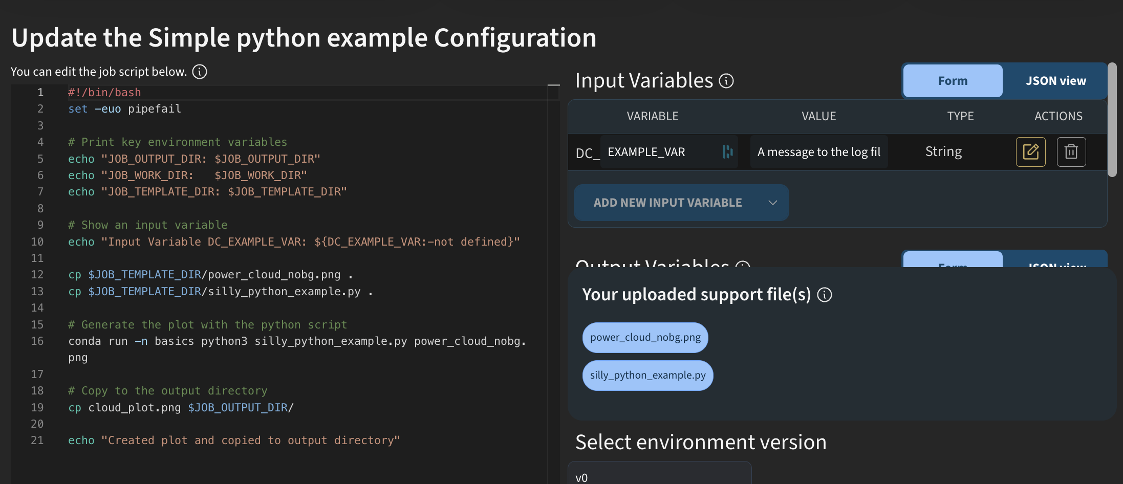
If we look at a simple Python example and view the template, you can see that everything is written in Bash. You had to explicitly call Python and include your own Python script, which you uploaded as a support file.

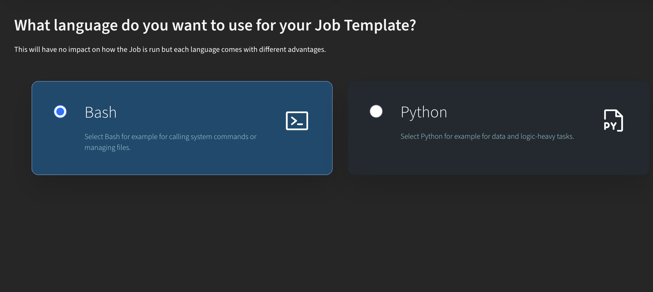
Now, let’s look at how this works with the new Python job type. I go to My Templates and click Create New Template. Here, you can choose between Bash (the traditional way of creating jobs) or Python.

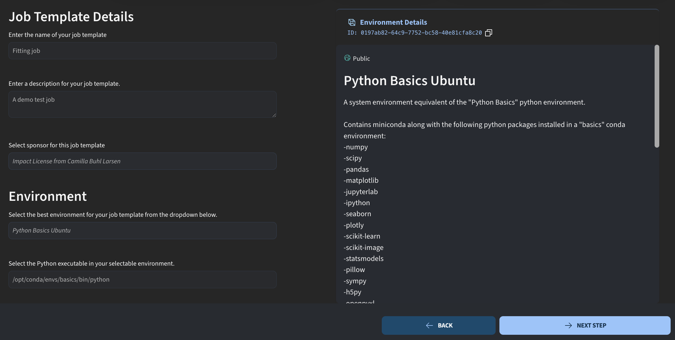
First, we define the job details. I give the job a name, for example a simple fitting script, and add a short description. As usual, we also specify who is sponsoring the job and select the environment.

Currently, Python jobs are still based on an Ubuntu environment. If you have built a custom Jupyter environment, you cannot select it here yet. I will therefore choose the Python Basics Ubuntu environment, which has a Conda environment installed that we can use to run this job.

The main difference for Python jobs appears here. You must define which Python executable should be used. This requires knowing a few details about the environment. An easy way to find the correct python executable path is to open a session with that environment and run which python.

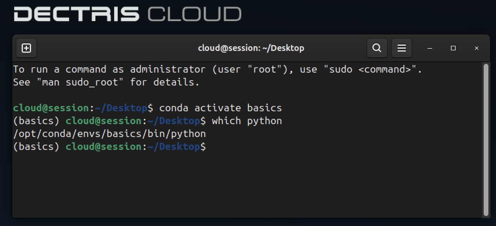
In this case, for the Basics Ubuntu environment, there is a Conda environment called basics, and this is the Python executable we will use.

/opt/conda/envs/basics/bin/python

I then click Next step.

This is what the Python job builder looks like. In the backend, this is still the same job engine as before: a Docker-based environment running a script. The difference is that the frontend now allows you to write Python code directly, without any Bash scripting.

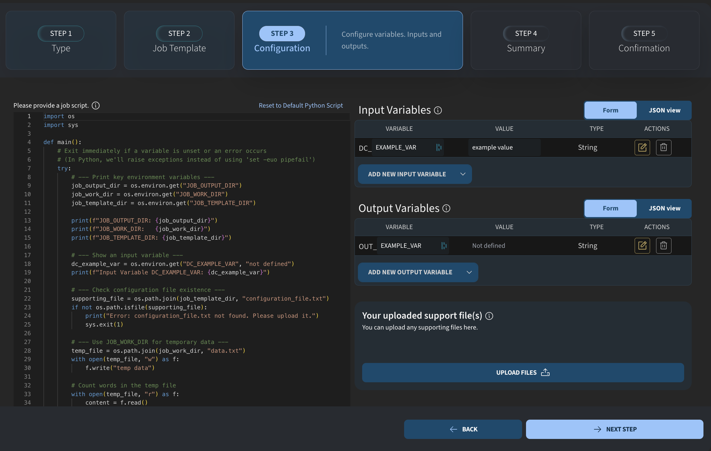
The overall logic is the same as for other jobs. You still have:

an output directory
a working directory
a template directory

The output directory contains files that will be available after the job has finished. The variable name is the same as in Bash jobs, and we use it to access the output directory inside the Python script via environment variables.

job_output_dir = os.environ.get("JOB_OUTPUT_DIR")

The template directory is where you can place any support files that you upload with the job.

job_template_dir = os.environ.get("JOB_TEMPLATE_DIR")

In this example, I will import a few packages. These packages must also be available in the environment you selected. I will import NumPy, Matplotlib for plotting, and the relevant module for performing a curve fit.

import numpy as np
import matplotlib.pyplot as plt
from scipy.optimize import curve_fit

I will keep these imports at the top and then add our own code below. Next, we define input variables. I remove the default variables and add new ones.

This script will fit some data, so I add a path variable called DC_DATA. I also add two string variables for axis labels.

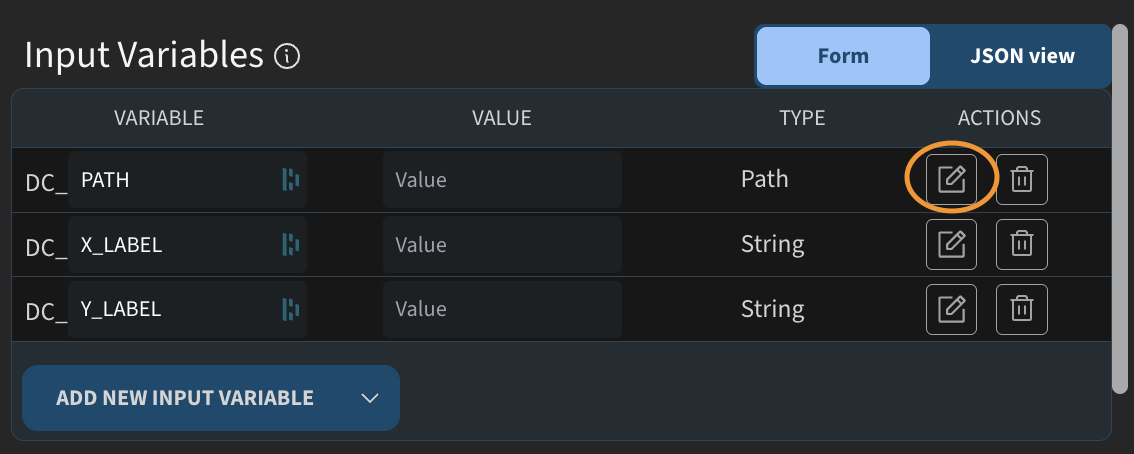
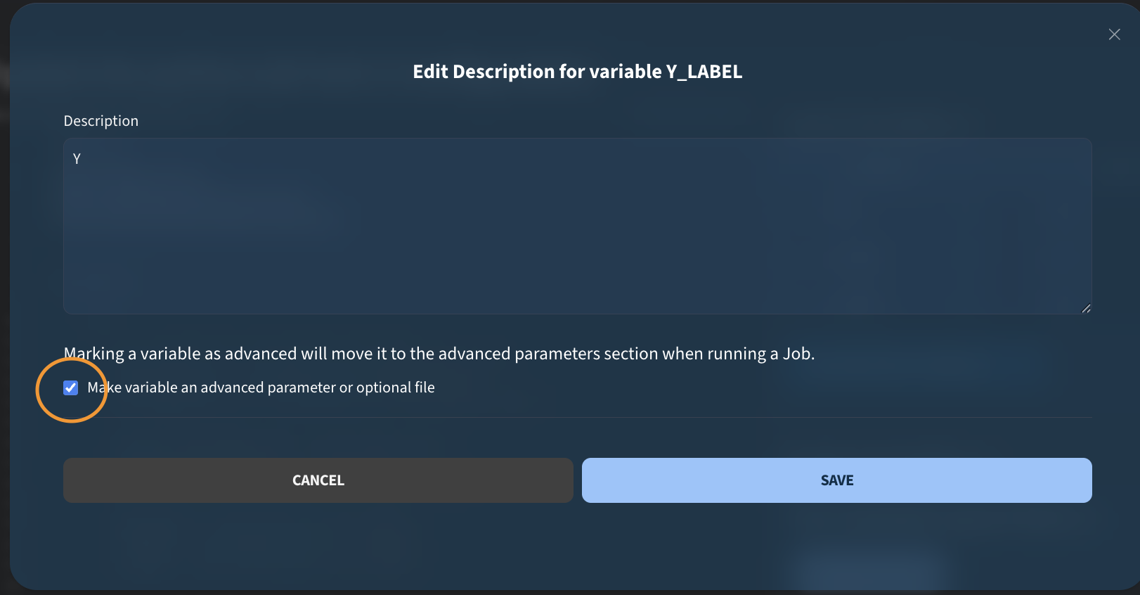
You may notice small icons next to the variables. As a job creator, you can add descriptions to provide context for users who run the job. For example, I can add a description like “Path to text file” and save it. I do the same for the other variables.

For one of the variables, I also mark it as advanced. We will see later how this affects the job execution interface.

These are our input variables. To use them in the Python script, we again read them from the environment. I add the corresponding code and make sure the variable names match.

data_path = os.environ.get("DC_PATH")
x_label = os.environ.get("DC_X_LABEL")
y_label = os.environ.get("DC_Y_LABEL")

Now we have the path to the data file and the two strings for the plot labels. The next step is to load the data and perform the fit. I load the data using NumPy’s loadtxt function and perform a simple linear fit.

x, y = np.loadtxt(data_path, unpack=True)
m, b = np.polyfit(x, y, 1)

I then create a plot using Matplotlib. I generate an array using linspace, plot the data, and overlay the fitted curve. The input string variables are used for labeling the axes, and the plot is shown at the end.

xx = np.linspace(x.min(), x.max(), 300)
plt.plot(x, y, "o", label="data")
plt.plot(xx, m*xx + b, "-", label=f"fit: y = {m:.3g}x + {b:.3g}")
plt.xlabel(x_label)
plt.ylabel(y_label)
plt.legend()
plt.show()

Finally, we want to save the plot so that it is accessible outside the job environment. To do this, I use the job output directory variable and combine it with a filename. I save the figure to this path. The saved figure will appear in the job output table once the job has completed.

output_file = os.path.join(job_output_dir, "fit_figure.png")
plt.savefig(output_file, dpi=300, bbox_inches="tight")

This is everything needed to define the job. It is a simple example, but it demonstrates the workflow. I click Next step and Start build, and the job template is saved immediately.

Running the Job

For reference, I am in Analysis → My Templates, and this is the fitting job I just created.

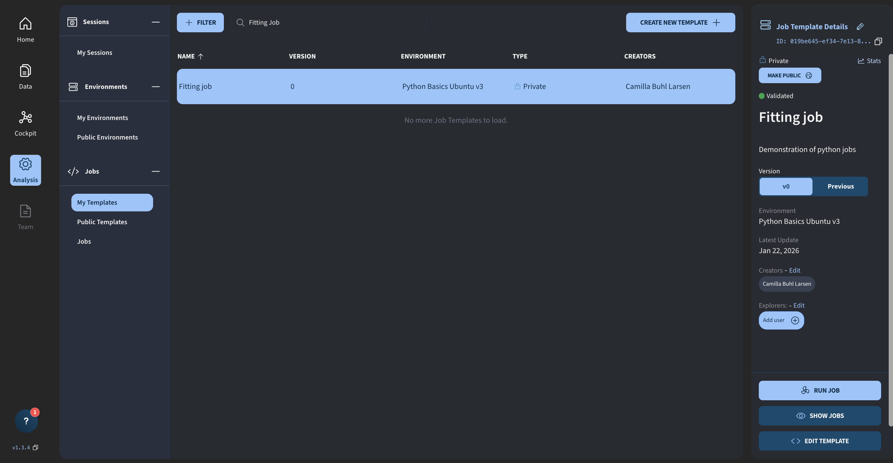
I click Run Job, and we now see the updated job execution interface.

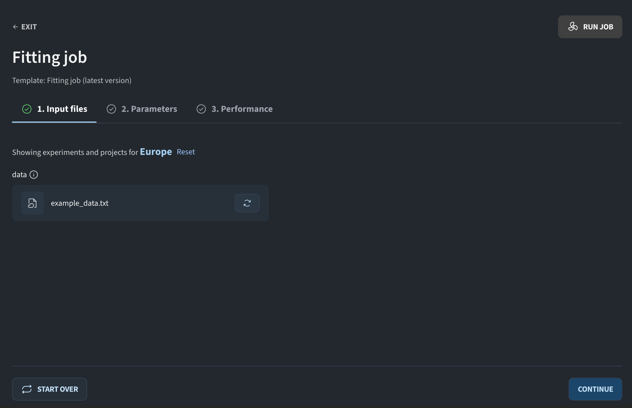
Previously, everything was shown on a single page. Now, the interface is split into several steps, giving each section more space.

The first step is configuring input files. This corresponds to the path variables defined in the job. I click Browse and select the data file. In my case, I go to Projects, choose the project Fitting Test, navigate to the raw directory, select the text file, and confirm. This is now the data that will be fitted.

I click Continue to configure parameters. For example, I set the X label to “X”. You may notice that the Y label is not visible. This is because it was marked as an advanced parameter. If I click Show advanced, it appears, and I can set its value as well.

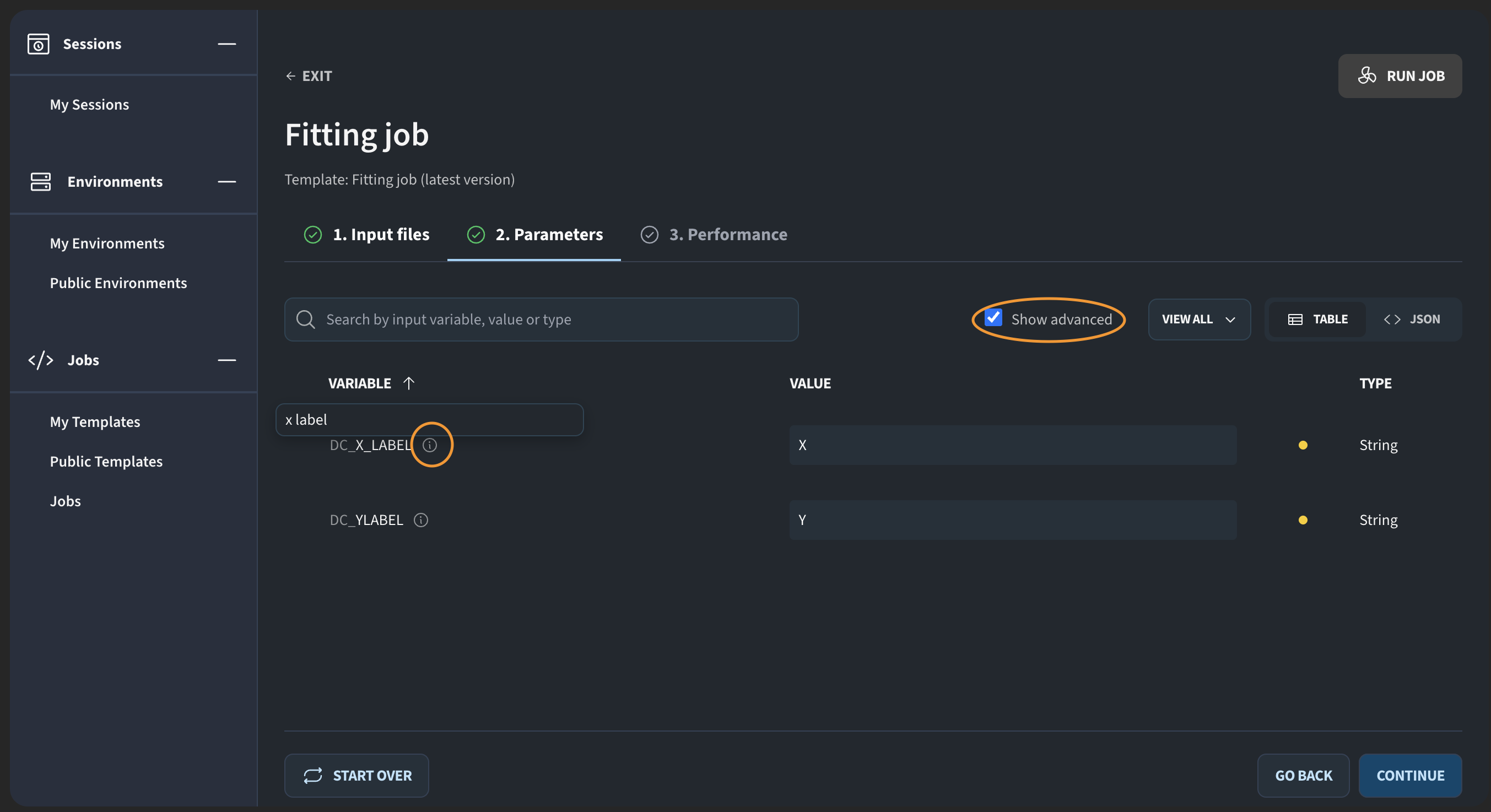
This is useful when you have parameters that only experienced users are likely to change, and you want to avoid overwhelming new users.

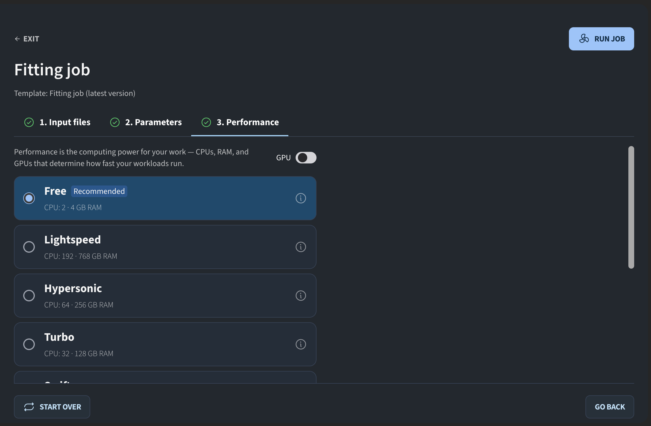
I click Continue. The final step is selecting the machine performance. I choose Free and then click Run Job. The job is now pending.

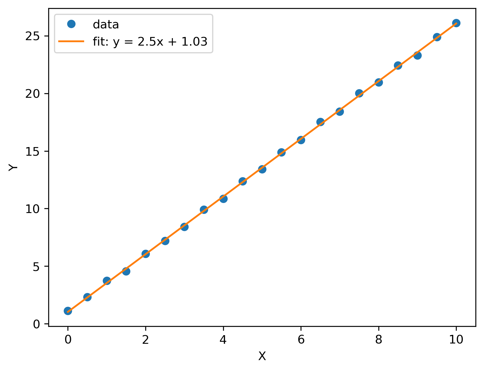
If we look at an earlier test run, this is the output you would get: the original data with a fitted curve plotted on top:

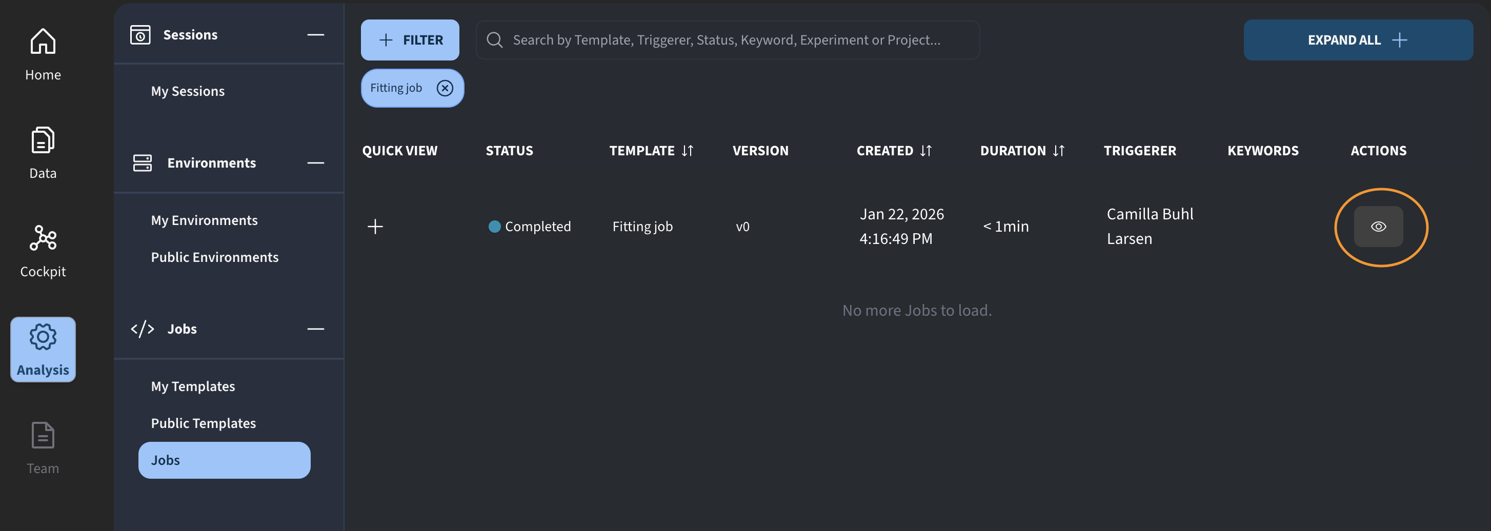
For the pending job, we can click the eye icon to review the inputs that were used.

This concludes a short update on the latest improvements to jobs on DECTRIS CLOUD. We are continuously improving this feature, so please feel free to reach out and share your feedback.

Summary: Example Job Template Script Shown During the Meeting

The job template was built with the Python Basics Ubuntu environment and defined with the following path to the python executable :

/opt/conda/envs/basics/bin/python

The script for performing a simple line fit and saving the plot to the output directory was :

import os
import sys
import numpy as np
import matplotlib.pyplot as plt
from scipy.optimize import curve_fit

def main():
    # Exit immediately if a variable is unset or an error occurs
    # (In Python, we'll raise exceptions instead of using 'set -euo pipefail')
    try:
        # --- Print key environment variables ---
        job_output_dir = os.environ.get("JOB_OUTPUT_DIR")
        job_work_dir = os.environ.get("JOB_WORK_DIR")
        job_template_dir = os.environ.get("JOB_TEMPLATE_DIR")

        print(f"JOB_OUTPUT_DIR: {job_output_dir}")
        print(f"JOB_WORK_DIR:   {job_work_dir}")
        print(f"JOB_TEMPLATE_DIR: {job_template_dir}")

        data_path = os.environ.get("DC_DATA")
        x_label = os.environ.get("DC_X_LABEL")
        y_label = os.environ.get("DC_Y_LABEL")

        x, y = np.loadtxt(data_path, unpack=True)
        m, b = np.polyfit(x, y, 1)

        xx = np.linspace(x.min(), x.max(), 300)
        plt.plot(x, y, "o", label="data")
        plt.plot(xx, m*xx + b, "-", label=f"fit: y = {m:.3g}x + {b:.3g}")
        plt.xlabel(x_label)
        plt.ylabel(y_label)
        plt.legend()
        plt.show()

        # Save
        output_file = os.path.join(job_output_dir, "fit_figure.png")
        plt.savefig(output_file, dpi=300, bbox_inches="tight")
        print("Job completed successfully.")

    except Exception as e:
        print(f"Error: {e}")
        sys.exit(1)

if __name__ == "__main__":
    main()

The input variables defined for the job (read as environment variables in the job script):

{
  "input_variables": {
    "DC_DATA": {
      "default_value": "",
      "type": "path",
      "description": "Path to text file"
    },
    "DC_X_LABEL": {
      "default_value": "",
      "type": "string",
      "description": "x label"
    },
    "DC_Y_LABEL": {
      "default_value": "",
      "type": "string",
      "description": "y label",
      "optional": true
    }
  }
}