GSAS-II batch refinement battery

Example of how one can run a GSAS-II refinement from a job template

Introduction

This job template has been created with the GSAS-II environment and has been created to run a batch refinement analysis on a battery reconstruction from a XRD-CT dataset. Details of the refinement script are given at the bottom of the page for anyone who wants to adapt it for their own refinement needs.

Quick start

To run this job, one needs to configure two paths in the job launcher:

DC_PATH: Path to .h5 file containing a series of powder profiles to be refined with Rietveld refinement. The .h5 file is expected to contain the fields "data" (size: nx, ny, nq) and "q" (size nq), where nx and ny are spatial dimensions of a reconstruction.
DC_CIF: Path to folder containing .cif files to be loaded during the refinement. For this specific case, the folder should contain al.cif, cu.cif, and fe.cif for the three crystallographic phases being refined.

Be aware that the job runs several refinements in parallel and will generate a number of temporary files that scales with the number of CPUs of the chosen machine type. If you choose a machine type with a lot of CPUs, make sure to increase the local software disk.

Output

The job script generates the following output:

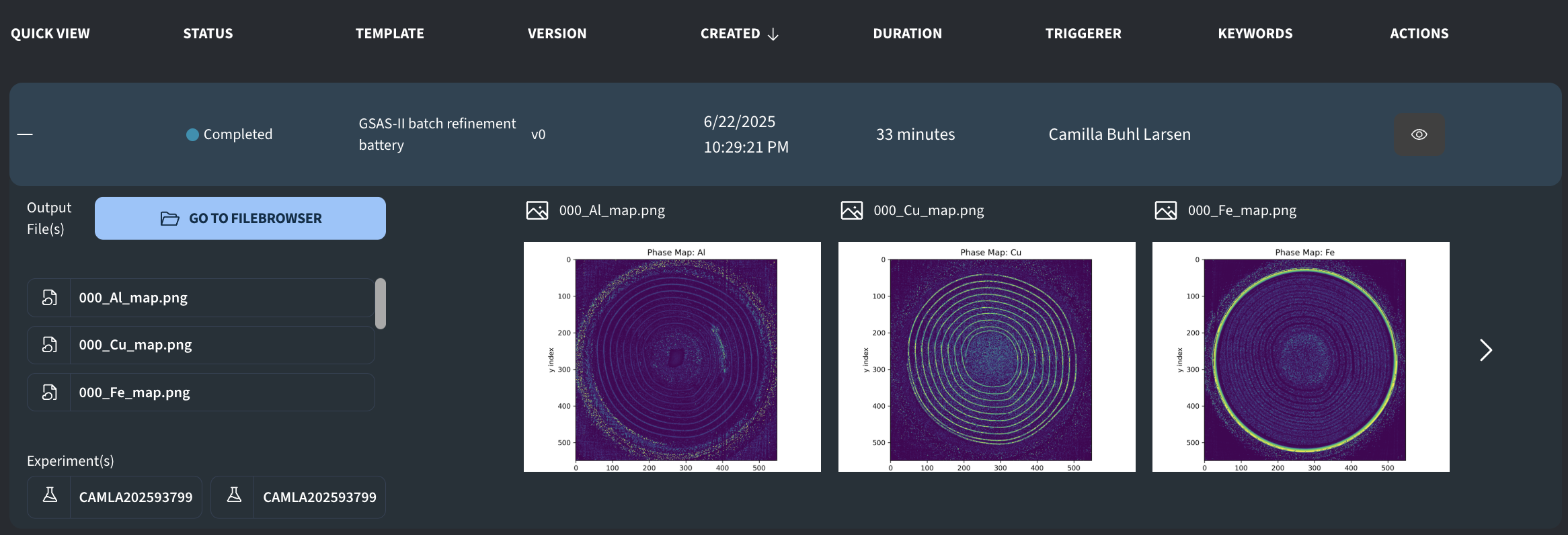
000_Al_map.png: Phase map of Al phase
000_Cu_map.png: Phase map of Cu phase
000_Fe_map.png: Phase map of Fe phase
Al_map.npy: Numpy array with fitted Al phase fractions
Cu_map.npy: Numpy array with fitted Cu phase fractions
Fe_map.npy: Numpy array with fitted Fe phase fractions
chi2data.npy: Numpy array with recorded chi2 as calculated in the script
chi2map.png: 2D map of fitted chi2

Job template configuration

Below we document the job and support python files used to run the job. These scripts can be adapted by anyone who wants to run their own GSAS-II refinement analysis in the cloud. Take note, that the above example only shows a rough way of getting the phase maps, and do not include any absorption corrections, instrument calibrations, etc:

Job script:

#!/bin/bash
set -euo pipefail

# Initialize conda 
source /home/cloud/gsas2full/etc/profile.d/conda.sh
conda activate base

# Print key environment variables
echo "JOB_OUTPUT_DIR: $JOB_OUTPUT_DIR"
echo "JOB_WORK_DIR:   $JOB_WORK_DIR"
echo "JOB_TEMPLATE_DIR: $JOB_TEMPLATE_DIR"
echo "DC_PATH: $DC_PATH"

cp $DC_CIF/*.cif .
cp $JOB_TEMPLATE_DIR/gsas2_batch_refinement.py .

python3 gsas2_batch_refinement.py $DC_PATH

cp *.png $JOB_OUTPUT_DIR
cp *.npy $JOB_OUTPUT_DIR

Support file: gsas2_batch_refinement.py:

import sys, os, h5py, contextlib, argparse, numpy as np
from multiprocessing import Pool, cpu_count
import matplotlib.pyplot as plt
from matplotlib.colors import LinearSegmentedColormap
sys.path.insert(0, '/home/cloud/gsas2full/GSAS-II/GSASII')
from GSASIIscriptable import G2Project
import time

# Get path
parser = argparse.ArgumentParser(description="Run GSAS-II refinements on hyperspectral powder dataset.")
parser.add_argument('data_path', type=str, help='Path to the .h5 file containing "data" and "q" arrays')
args = parser.parse_args()
data_path = args.data_path

start = time.perf_counter()

# wavelength
lam = 0.11979

# Simple instrument configuration
inst_vals = {
    'Type': ['PXC', 'PXC', False],
    'Lam': [lam, lam, False],
    'Zero': [0.0, 0.0, False],
    'Polariz.': [0.0, 0.0, False],
    'U': [0.01, 0.01, False],
    'V': [0.0, 0.0, False],
    'W': [0.01, 0.01, False],
    'X': [0.0, 0.0, False],
    'Y': [0.0, 0.0, False],
    'SH/L': [0.002, 0.002, False]
}
inst_flags = {k: False for k in inst_vals}
inst_tuple = (inst_vals, inst_flags)

def refine_slice(args):
    y, x, qvec, intensity = args
    # 1) write your slice file
    fn = f"slice_{y}_{x}.xy"
    twotheta = 2*np.degrees(np.arcsin(qvec*lam/(4*np.pi)))
    np.savetxt(fn, np.column_stack((twotheta, intensity.clip(min=0))),
               header="2theta Intensity")
    # 2) build a one‐histogram project
    gpx_path = f"slice_{y}_{x}.gpx"
    proj = G2Project(newgpx=gpx_path)
    # open null-device once (to supress stdout so log file does not get huge)
    with open(os.devnull, 'w') as devnull, \
        contextlib.redirect_stdout(devnull), \
        contextlib.redirect_stderr(devnull):


        hist = proj.add_powder_histogram(fn, iparams=inst_tuple)

        # Add phases: Have a few for now, more can be added for accuracy
        for cif, name in [('fe.cif','Fe'),
                          ('cu.cif','Cu'),
                          ('al.cif','Al')]:
            proj.add_phase(cif, phasename=name)
            phase = proj.phase(name)
            proj.link_histogram_phase(hist, phase)
            phase.data['Histograms'][hist.name]['Scale'] = [1.0, True]
            #phase.set_refinements({'Cell': True})

        hist.data['Background'][0][3]           = 0.0
        hist.data['Sample Parameters']['Scale'] = [1.0, False]

        proj.set_Controls('cycles', 20)
        proj.do_refinements([{}])

    # 3) pull out GOF
    res   = hist.residuals
    rwp   = res.get('wR')     or 0
    rexp  = res.get('wRmin')  or 1
    chi2  = (rwp/rexp)**2

    # 4) pull out each scale
    scales = {ph.name: ph.data['Histograms'][hist.name]['Scale'][0]
              for ph in proj.phases()}
    #print(f"x={x}, y ={y}, chi2={chi2}, scales={scales}")

    # Delete temporary files (slice, project file) or will run out of disk space
    os.remove(fn)
    os.remove(gpx_path)
    os.remove(gpx_path.replace(".gpx", ".lst"))
    return y, x, chi2, scales

# Load data
with h5py.File(data_path, 'r') as hf:
    qvec = hf['q'][:]
    vol  = hf['data'][:]

ny, nx, nq = vol.shape
coords = [(y, x, qvec, vol[y,x,:])
          for y in range(ny) for x in range(nx)]

phase_maps = {p: np.zeros((ny,nx)) for p in ['Fe','Cu','Al']}
chi2map    = np.zeros((ny,nx))

# spawn a pool and do the refinements, we use all available cpus
n_procs = cpu_count()
print(f"Starting refinement with {n_procs} processes")
with Pool(processes=n_procs) as pool:
    for y, x, chi2, scales in pool.imap_unordered(refine_slice, coords):
        chi2map[y,x] = chi2
        if chi2 < 1:
            for ph, val in scales.items():
                phase_maps[ph][y,x] = val
        else:
            # leave phase_maps[*][y,x] = 0
            pass

# now plot / np.save
chi2map[chi2map==1]=0

for phase_name, phase_data in phase_maps.items():
    plt.figure(figsize=(6, 5))
    a = np.percentile(phase_data[phase_data>0],98)
    phase_data[phase_data>a]=0
    plt.imshow(phase_data, vmin=np.percentile(phase_data[phase_data>0],25), vmax=np.percentile(phase_data[phase_data>0],99))
    plt.title(f"Phase Map: {phase_name}")
    plt.xlabel("x index")
    plt.ylabel("y index")
    plt.tight_layout()

    # Save as PNG and NPY
    output_path = os.path.join(f"000_{phase_name}_map.png")
    plt.savefig(output_path, dpi=300)
    plt.close()  # Close figure to avoid memory buildup
    npy_path = f"{phase_name}_map.npy"
    np.save(npy_path, phase_data)

plt.figure(figsize=(6,5))
plt.imshow(chi2map, origin="lower", cmap="Greys")
plt.title("Chi2 map")
plt.tight_layout()
plt.savefig("chi2map.png", dpi=300)
plt.close()
np.save("chi2data.npy", chi2map)

total_sec = time.perf_counter() - start
print(f"Total refinement time: {total_sec:.1f} s "
      f"({total_sec/60:.1f} min, {total_sec/3600:.2f} h)")

Versions

Version 0

Initial version created with version 1 of the GSAS-II environment