Use case: XRD-CT battery analysis

This use case shows an example of how XRD-CT data can be analyzed and used to generate rough phase maps

Data and software used

Sinogram data from: Vamvakeros, A., Matras, D., Ashton, T. E., Dong, H., Bauer, D., Odarchenko, Y., Price, S. W. T., Butler, K. T., Gutowski, O., Dippel, A.-C., von Zimmermann, M., Darr, J., Jacques, S. D. M., & Beale, A. M. (2021). Cycling Rate-Induced Spatially-Resolved Heterogeneities in Commercial Cylindrical Li-Ion Batteries: Datasets [Data set]. Zenodo. https://doi.org/10.5281/zenodo.5172980
Paper based on example data: A. Vamvakeros, D. Matras, T. E. Ashton, A. A. Coelho, H. Dong, D. Bauer, Y. Odarchenko, S. W. T. Price, K. T. Butler, O. Gutowski, A. C. Dippel, M. v. Zimmerman, J. A. Darr, S. D. M. Jacques, A. M. Beale, Cycling Rate-Induced Spatially-Resolved Heterogeneities in Commercial Cylindrical Li-Ion Batteries. Small Methods 2021, 5, 2100512. https://doi.org/10.1002/smtd.202100512
Fiji (ImageJ): Schindelin, J., Arganda-Carreras, I., Frise, E., Kaynig, V., Longair, M., Pietzsch, T., … Cardona, A. (2012). Fiji: an open-source platform for biological-image analysis. Nature Methods, 9(7), 676–682. doi:10.1038/nmeth.2019
nDTomo: Vamvakeros, A., Papoutsellis, E., Dong, H., Docherty, R., Beale, A.M., Cooper, S.J., Jacques, S.D.M.J., nDTomo: A Python-Based Software Suite for X-ray Chemical Imaging and Tomography, 2025, https://doi.org/10.26434/chemrxiv-2025-h5t2x
GSAS-II Toby, B. H., & Von Dreele, R. B. (2013). “GSAS-II: the genesis of a modern open-source all purpose crystallography software package”. Journal of Applied Crystallography, 46(2), 544-549. doi:10.1107/S0021889813003531

DECTRIS CLOUD environments

Fiji (ImageJ) v0
nDTomo v0
nDTomo Jupyter Notebook v0
GSAS-II v1

Processing steps

1. Project creation and data upload

Create a project by navigating to Data → My Projects → Add Project + and fill out the metadata:

Navigate inside the project space and upload the following .h5 files from the zenodo repository:

2. Data visualization in ImageJ

To look at the data with ImageJ, you can use the public Fiji (ImageJ) environment to start a session.

To start a session, navigate to Analysis → Public Environments and search for Fiji. Click on the Fiji environment card and then START SESSION in the new panel that pops out from the side.

On the following page, the Fiji environment will be preselected. Configure your session by choosing a name, local software disk (space needed for the installed software, not the data in the cloud, for Fiji 16 GB is enough), and the sponsor.

Finally choose the performance in the right panel before clicking NEXT STEP. This brings you to a page where you can select your created project.

Once inside the virtual machine, you can start ImageJ by going to the the Fiji.app folder in the home directory:

When opening the files with the hdf5 reader plugin, you can find them by navigating to the Desktop and going along the /dectris_data/ path.

3. Preprocessing with nDTomo in a python environment

To process the sinograms, you can start a session with the nDTomo Jupyter environment.

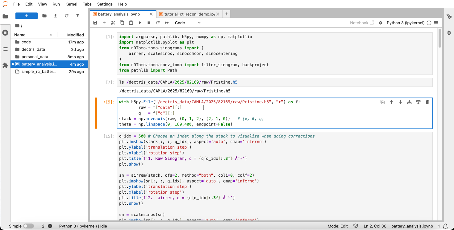
Within the session, you can start a new notebook and use the following code for processing the sinograms. Feel free to experiment with improving the preprocessing steps:

import argparse, pathlib, h5py, numpy as np, matplotlib
import matplotlib.pyplot as plt
from nDTomo.tomo.sinograms import (
    airrem, scalesinos, sinocomcor, sinocentering
)
from nDTomo.tomo.conv_tomo import filter_sinogram, backproject
from pathlib import Path

Import your uploaded sinogram data from your project. Make sure to adjust the path to match the mounted file path of your project:

with h5py.File("/dectris_data/CAMLA/2025/82169/raw/Pristine.h5", "r") as f:
        raw = f["data"][:]         
        q   = f["q"][:]
stack = np.moveaxis(raw, (0, 1, 2), (2, 1, 0))   # (x, θ, q)
theta = np.linspace(0, 180,400, endpoint=False)

The moveaxis command is used to make sure that the data is arranged in the way that nDTomo expects.

We can now perform the preprocessing steps:

q_idx = 500 # Choose an index along the stack to visualize when doing corrections
plt.imshow(stack[:, :, q_idx], aspect='auto', cmap='inferno')
plt.ylabel('translation step')
plt.xlabel('rotation step')
plt.title(f'1. Raw Sinogram, q = {q[q_idx]:.3f} Å⁻¹')
plt.show()

sn = airrem(stack, ofs=2, method="both", coli=0, colf=2)
plt.imshow(sn[:, :, q_idx], aspect='auto', cmap='inferno')
plt.ylabel('translation step')
plt.xlabel('rotation step')
plt.title(f'2.  airrem, q = {q[q_idx]:.3f} Å⁻¹')
plt.show()

sn = scalesinos(sn)
plt.imshow(sn[:, :, q_idx], aspect='auto', cmap='inferno')
plt.ylabel('translation step')
plt.xlabel('rotation step')
plt.title(f'3. scalesinos, q = {q[q_idx]:.3f} Å⁻¹')
plt.show()

sn = sinocomcor(sn, interp=False)
plt.imshow(sn[:, :, q_idx], aspect='auto', cmap='inferno')
plt.ylabel('translation step')
plt.xlabel('rotation step')
plt.title(f'4. sinocomcor, q = {q[q_idx]:.3f} Å⁻¹')
plt.show()

sn = sinocentering(sn, crsr=20, interp=True, scan=180, channels=None, pbar=False)
plt.imshow(sn[:, :, q_idx], aspect='auto', cmap='inferno')
plt.ylabel('translation step')
plt.xlabel('rotation step')
plt.title(f'5. sinocentering, q = {q[q_idx]:.3f} Å⁻¹')
plt.show()

Perform reconstruction of just a single slice:

sino = sn[:, :, q_idx]
sino_f = filter_sinogram(sino, filter_type="Ramp")
test = backproject(sino_f, theta)
plt.imshow(test)

Once satisfied with the above test, you can loop over all q-indices and make a reconstruction for each:

nx, ntheta, nq = sn.shape             
vol = np.empty((nx, nx, nq), dtype="float32")

for j in range(nq):
    sino = sn[:, :, j] 
    sino_f = filter_sinogram(sino, filter_type="Ramp")
    vol[:, :, j] = backproject(sino_f, theta)
    if j % 100 == 0:
        print(f"reconstructed {j}/{nq}")

Make sure to save your reconstruction results in a .h5 file, if you want to continue the analysis within a different environment. In this case, the .h5 file is saved to the work directory of my project. Make sure to adjust the path to your own personal project folder:

with h5py.File('/dectris_data/CAMLA/2025/82169/work/simple_rc_battery.h5', 'w') as hf:
    hf.create_dataset('q', data=q)
    hf.create_dataset('data', data=vol)

4. Starting the nDTomo GUI

If you want to proceed the analysis using the nDTomo GUI, you can start up the nDTomo environment. This environment differ from the previous one by being a system environment, meaning that you within the virtual machine will have access to an Ubuntu system, where the nDTomo components are installed.

5. Configuring a job to run batch refinements with GSAS-II

As a final step, we will perform a Rietveld refinement of every spectrum in the .h5 file.

This can be done by making use of the public GSAS-II batch refinement battery job template created for this use case.

To run the job, we need to provide a path to the reconstructed .h5 file from the previous step, as well as a path to a folder containing the .cif files for the phases we are refining (Al, Cu, Fe).

Before running the job, we therefore upload the files al.cif, cu.cif and fe.cif to the work folder in our project. The GSAS-II refinement job will look for these specific files when starting the refinement.

Once this is done, you can access and run the job template by going to Analysis → Public Job Templates and choosing the GSAS-II batch refinement battery job template:

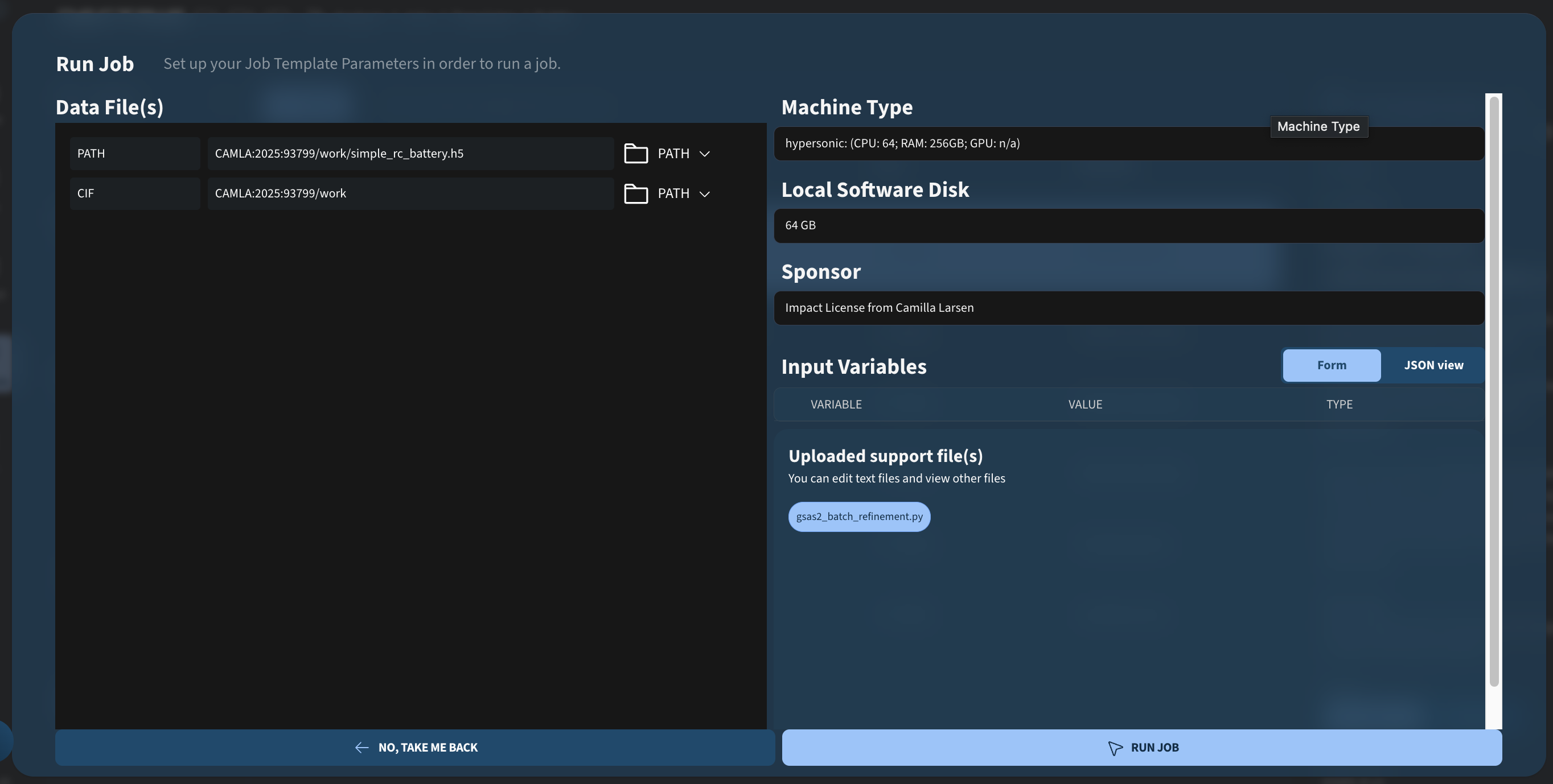
After running it, you should see the following output:

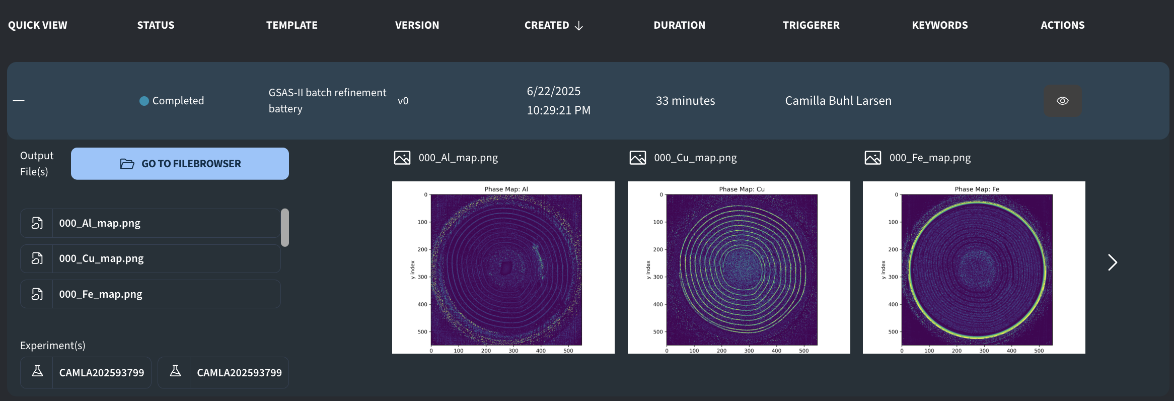
The job template attempts to parallelize the refinements, meaning that the running time should decrease with more powerful machine types. The above results were achieved with a Hypersonic node (64 CPUs) and took 33 minutes, while a test run with the Turbo node (32 CPUs) took 51 minutes.

6. Getting access to the demonstration project

If you want to be added to the example project for the video, so you do not have to run the full reconstruction yourself, you can contact us at support@dectris.cloud