UC #1 : The XDS Reproducibility Project

Speaker: Clemens Vonrhein - Global Phasing

Learning objectives

By the end of this workshop you will have:

Run the same dataset through both the standalone XDS job template and the autoPROC job template on DECTRIS D.LAB, and compared the results.
Learned how to override individual XDS.INP parameters through the job template, without editing the file by hand.
Seen how D.LAB captures the full context of a job — input data, software version, environment, parameters, and outputs — so any result can be traced back and reproduced.

Available Datasets

You will have access to the following datasets on DECTRIS D.LAB during the workshop:

5RET (https://zenodo.org/records/3730992)
5RE4 (https://zenodo.org/records/3730483)
5RG0 (https://zenodo.org/records/3731556)
5RFL (https://zenodo.org/records/3731412)
5REK (https://zenodo.org/records/3730929)
5RE7 (https://zenodo.org/records/3730531)

The datasets will be available in you given project under raw/UC1_XDS_Reproducibility

Choose one dataset for your group to focus on.

DECTRIS D.LAB Job Templates

xds_par & generate_XDS.INP - runs XDS directly from a supplied or auto-generated XDS.INP.

autoPROC process workshop - runs autoPROC's process command, which wraps XDS together with scaling, symmetry determination, and STARANISO anisotropic analysis. (The template will be made available during the workshop)

Part 1: A first run with XDS

Running the XDS template

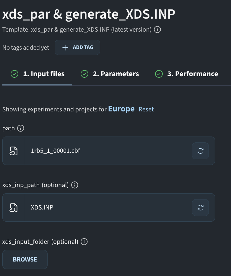
Go to the xds job template.
Configure the path to the first image file of your chosen dataset.
Configure DC_XDS_INP_PATH to point at the XDS.INP file for your dataset, found under auxiliary/UC1_XDS_Reproducibility/SAMPLE/XDS.INP. This file specifies how xds_par should run.
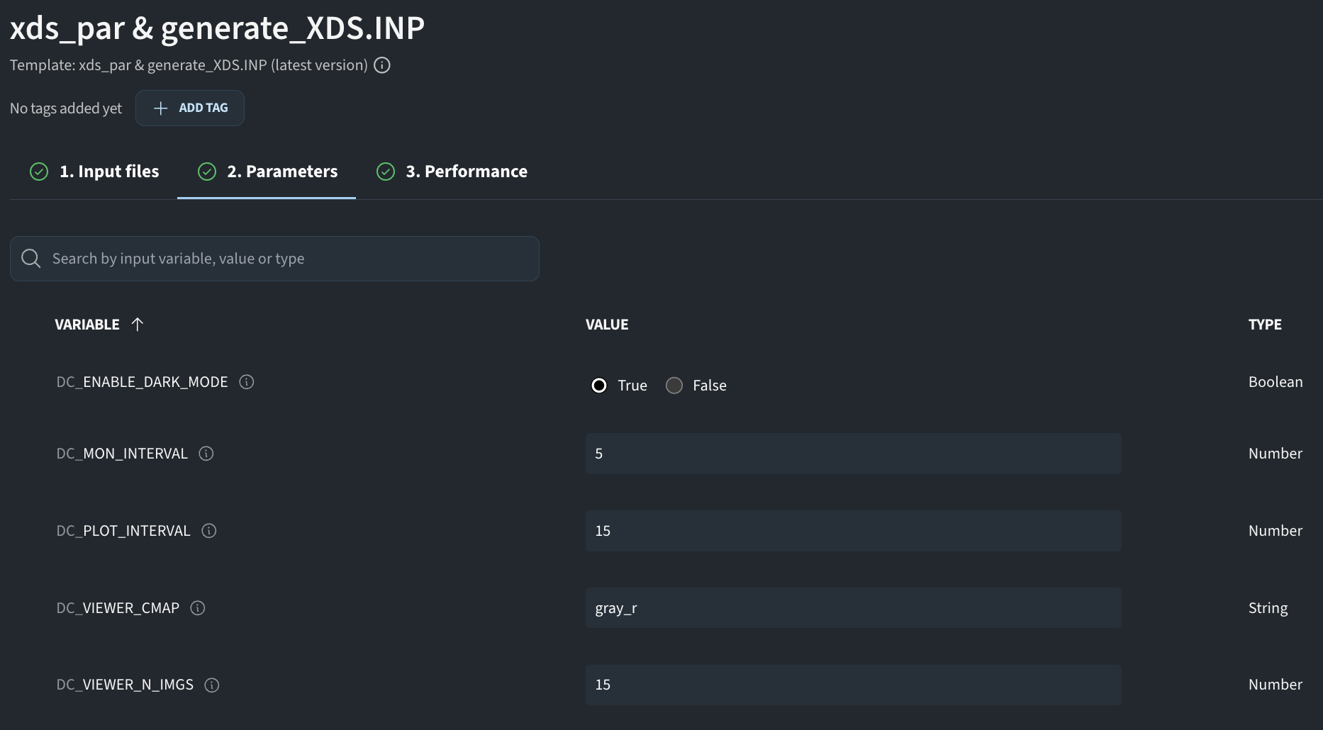
Leave DC_XDS_INPUT_FOLDER empty. It's only used to continue from an earlier analysis (e.g. reusing an existing SPOT.XDS/XPARM.XDS) — not needed for a first run.
On the Parameters tab, leave every input at its default value for this first run.
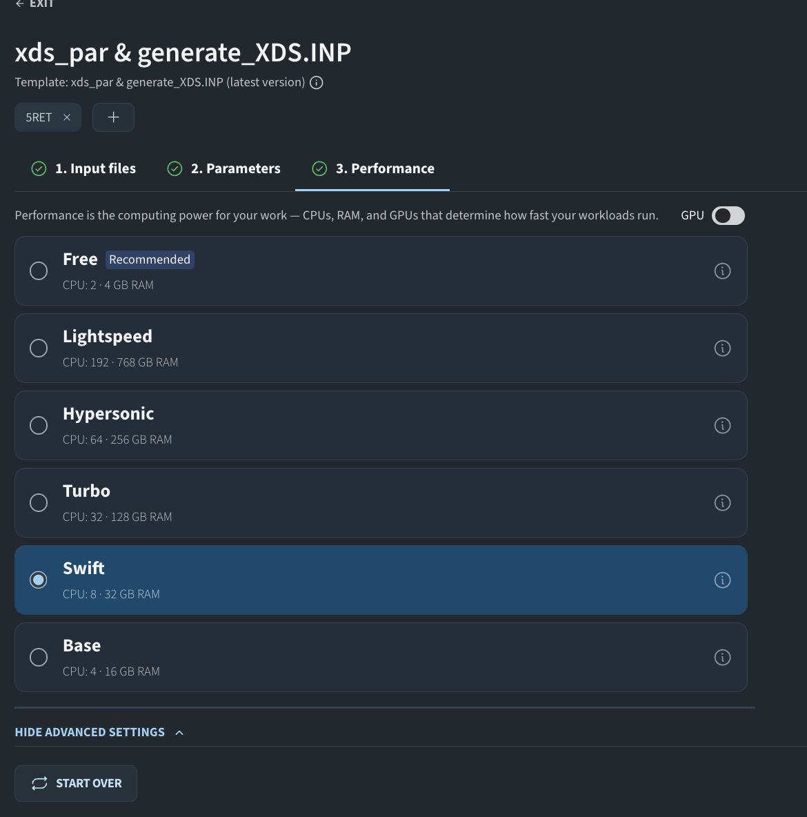
On the Performance tab, select the base machine (4 CPU, 16 GB RAM) — sufficient for the datasets in this workshop.
Click on the ADD TAG button and write your sample name. This will help you organize your results in your Analysis Overview.
Click RUN JOB. You can follow its progress from Analysis → Overview.

Inspecting the job details page

The job details page has several tabs:

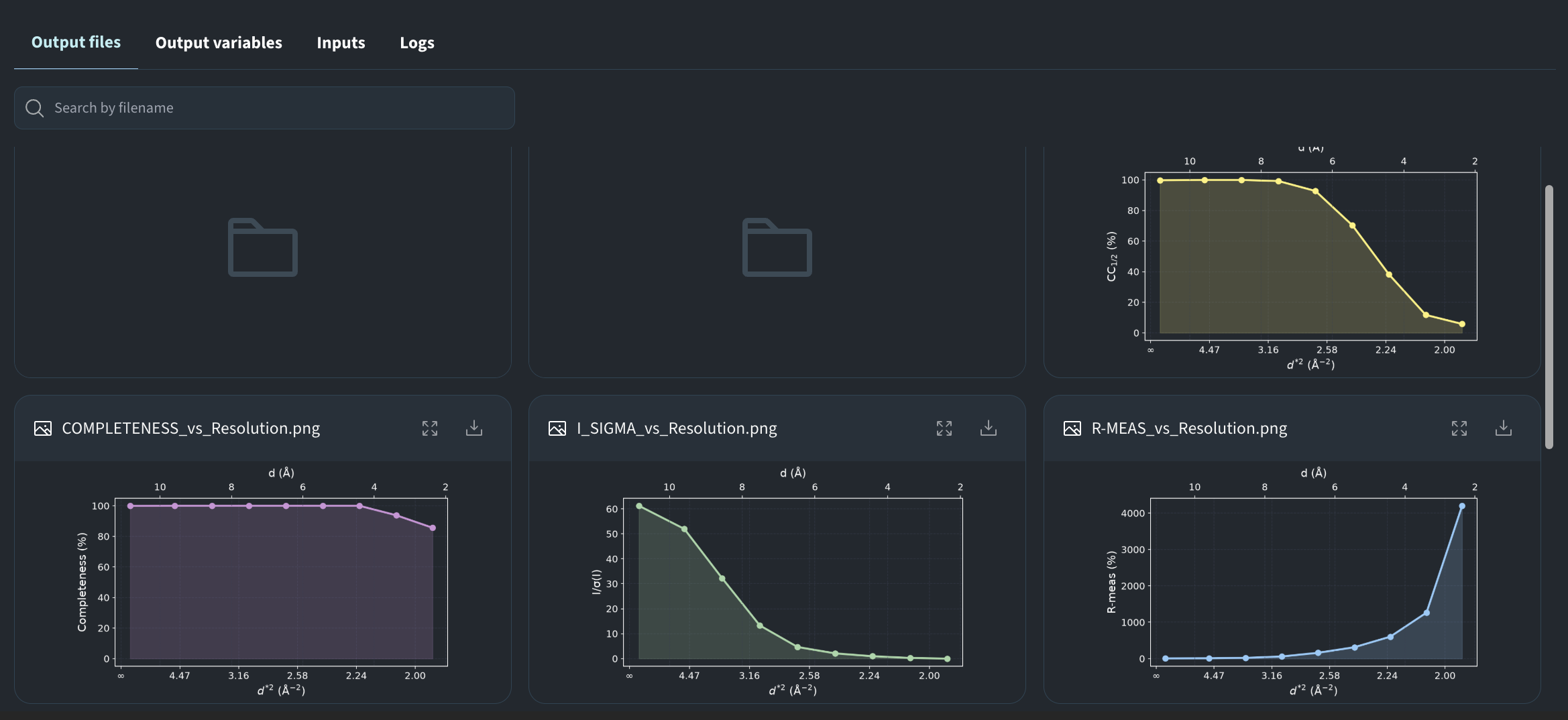
Output files — every file generated during the run, including the generated quality plots.
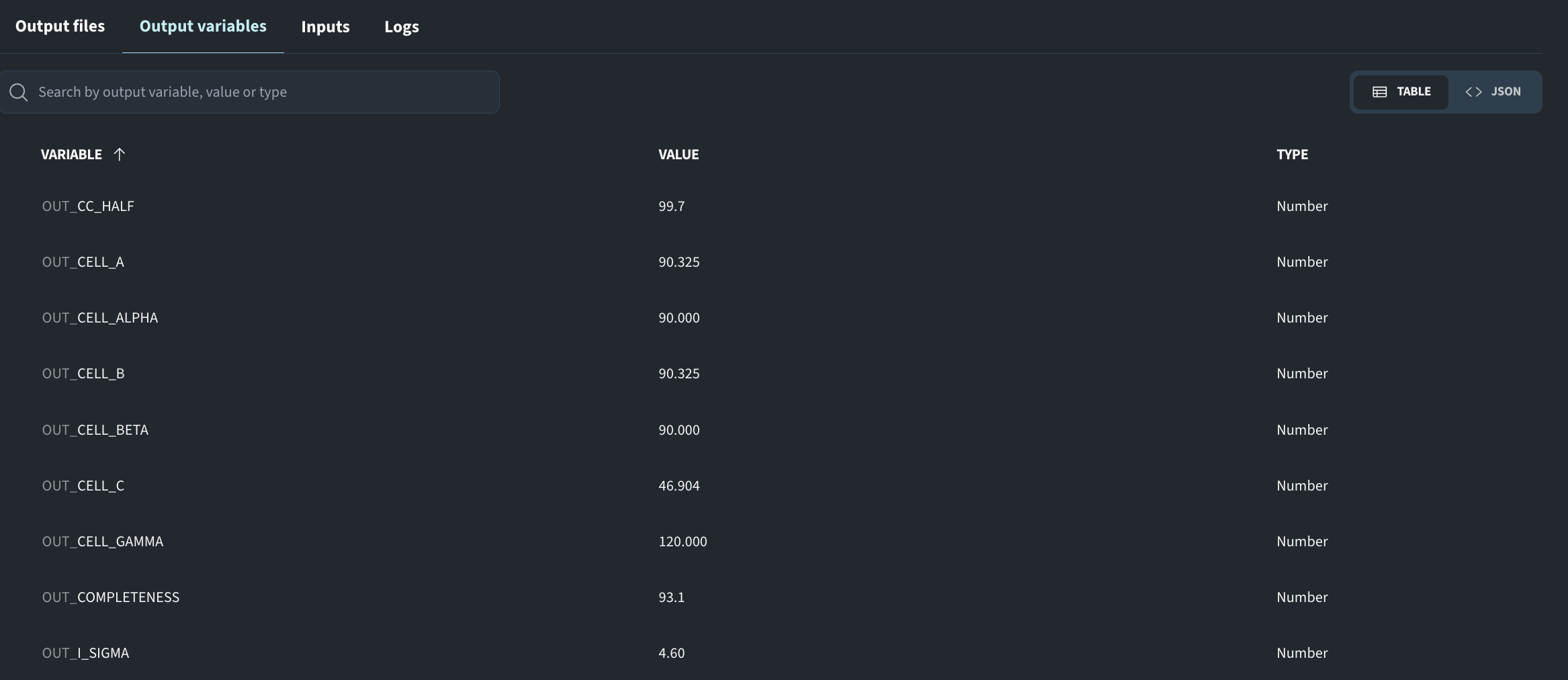
Output variables — parameters extracted from the job's output, such as refined cell constants.
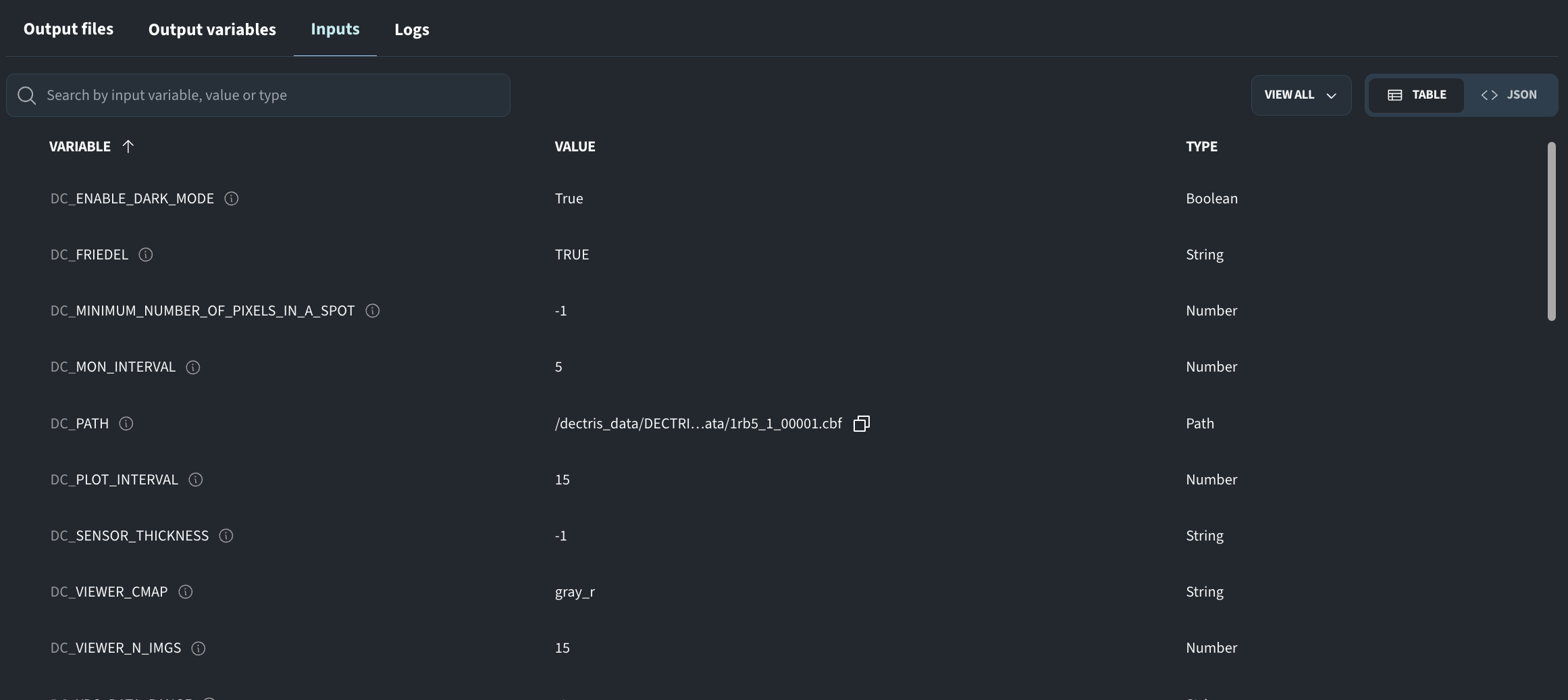
Inputs — every input parameter used for this run. Keeping this context means you can always trace back exactly how a result was produced.
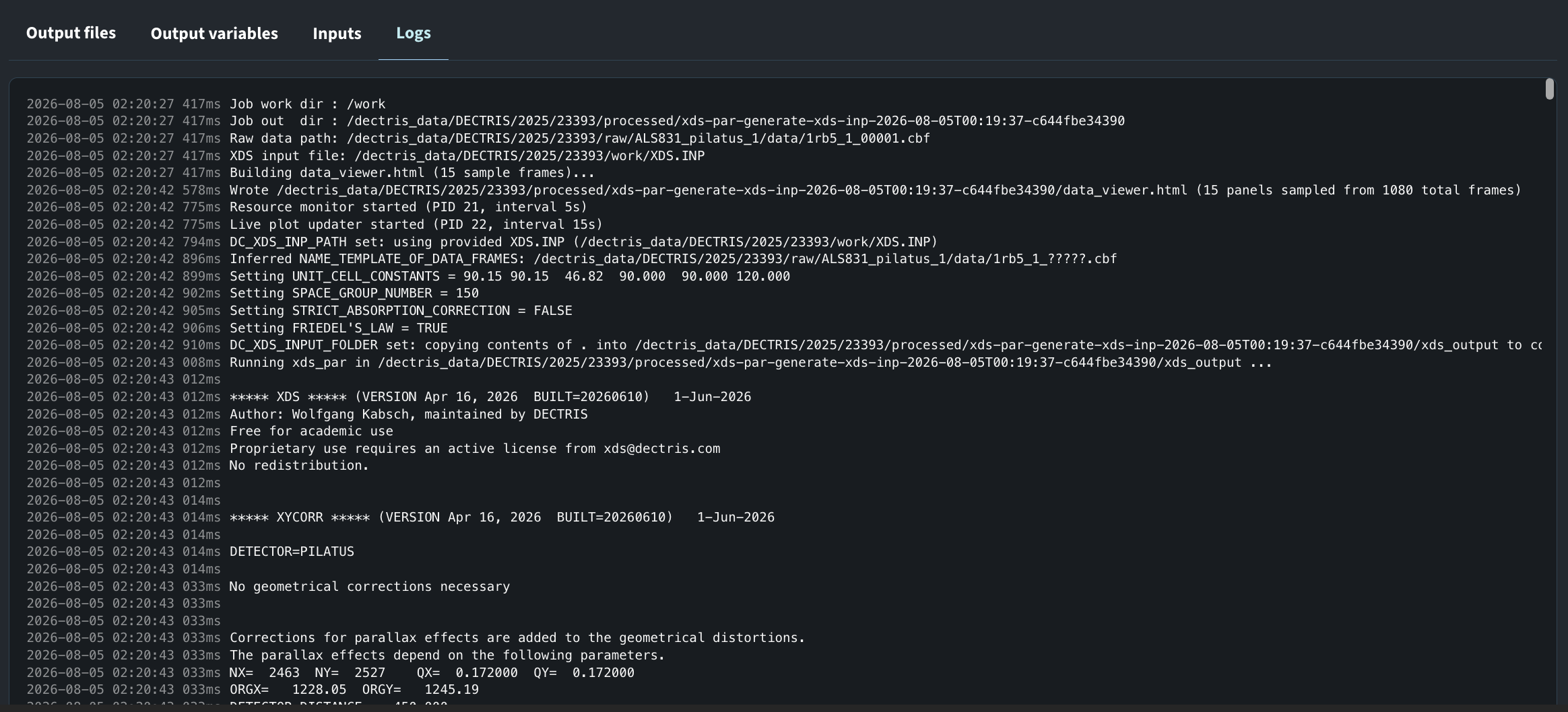
Logs — everything written to stdout during the job.

Having a look at the raw data

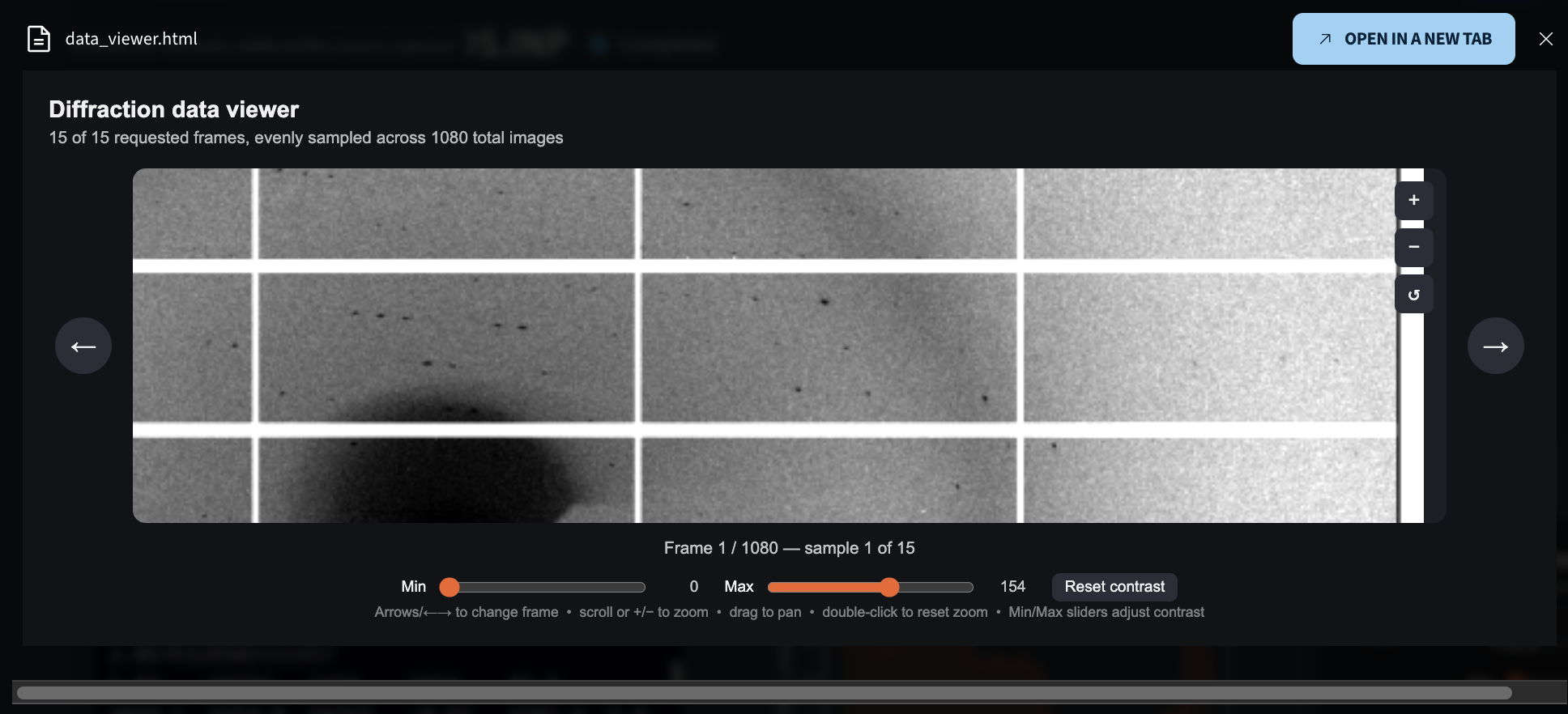
The output includes data_viewer.html — open it to page through a sample of raw frames from the dataset. This is a chance to check spot shape and spot any features in the data that may have affected the processing. The viewer supports scroll-to-zoom, click-and-drag panning, and Min/Max sliders to adjust contrast on the fly, so you can inspect faint features or an overexposed frame without needing to reprocess anything.

Look at the raw XDS output

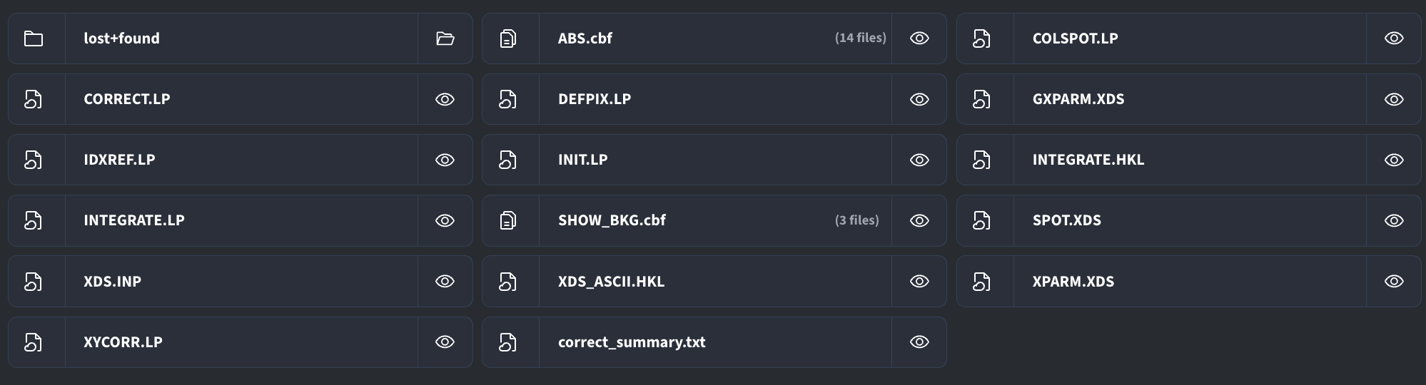
Beyond the summary quality plots, you can inspect XDS's own output files directly: from the Output files tab, open the xds_output folder to see every file XDS generated, plus the exact XDS.INP used for the run.

The various .LP files show, step by step, how indexing, integration, and scaling went.

Part 2: Running autoPROC

Running the autoPROC template

Go to the autoPROC process workshop job template.
On the first page, point it at the folder containing your chosen sample's data.
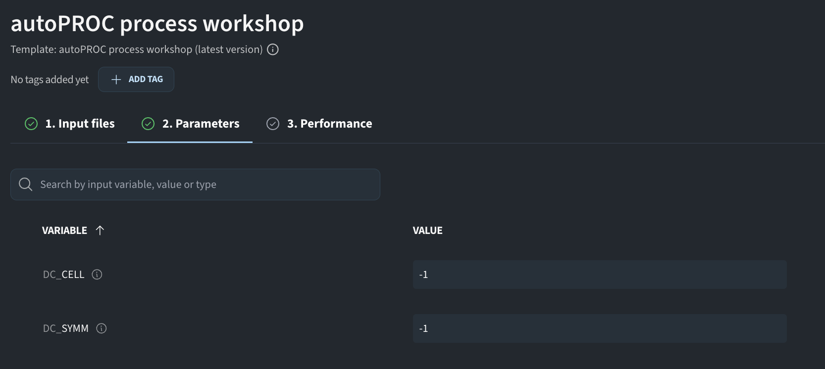
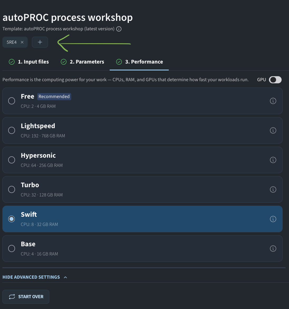
On the Parameters page, leave DC_CELL and DC_SYMM at -1 — this tells autoPROC to determine both automatically.
On the last page, choose the same base machine type as before.
Add a tag with your sample name, either before or after starting the job.
Click RUN JOB.

Inspecting the output

In the job output folder, all output files generated by autoPROC can be found in the autoPROC subfolder. In addition, the main output folder also contains a file 0_autoPROC_summary.html, which can be opened to view a report of the autoPROC analysis. If you click on the OPEN IN A NEW TAB button, you can get a full-page view of the html report:

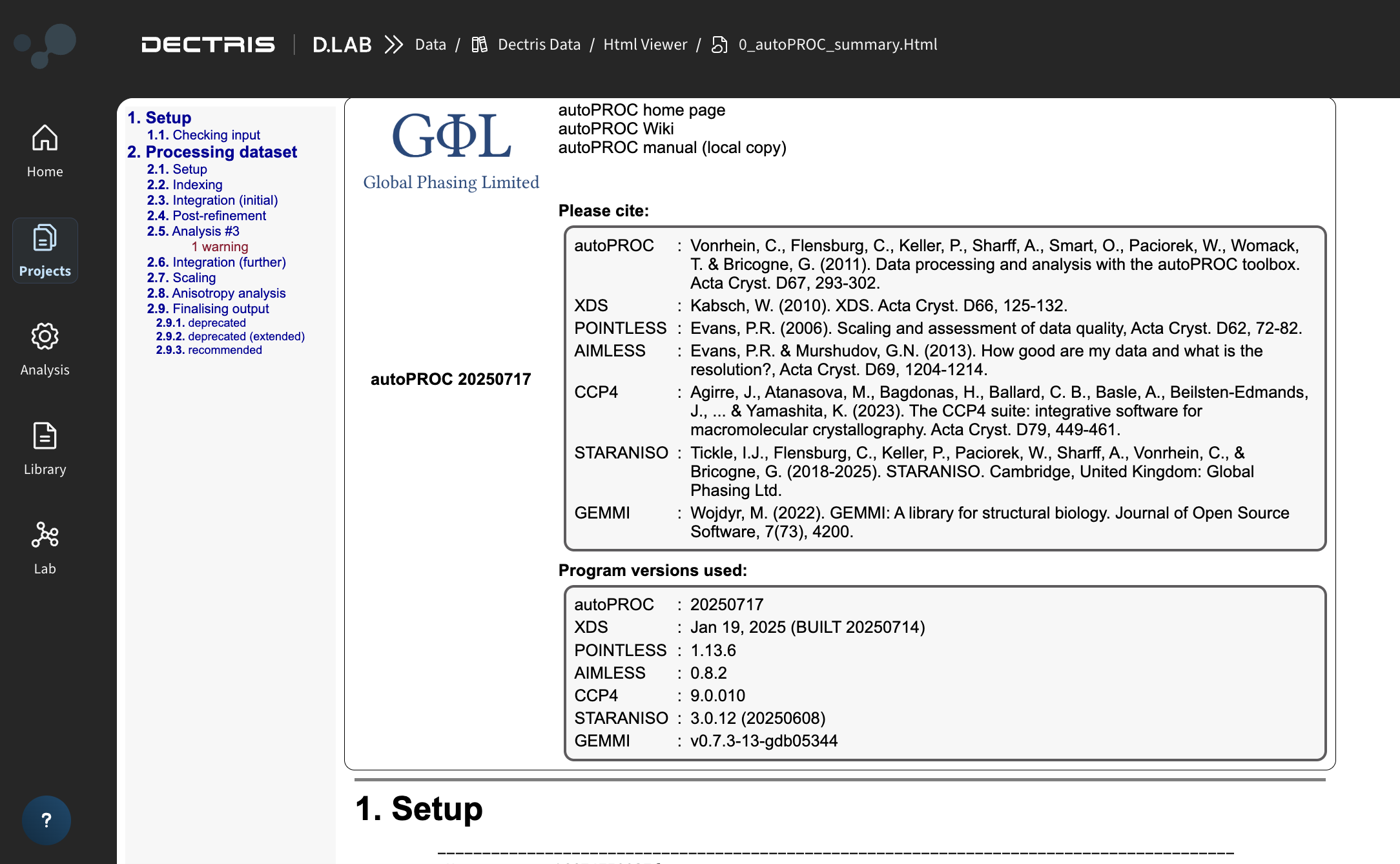
The html can also be downloaded and opened in a browser of your own choosing. Note however, that in either case the hyperlinks will not work.

Discussion prompt: Differences in XDS and autoPROC output

What were the differences in the XDS output vs the autoPROC output ?
How does the XDS.INP differ between the two jobs ?
Did autoPROC flag any warnings, which you did not take into consideration in the XDS job?

Part 3: Re-running the XDS job

Based on the discussion above: what would you change in your XDS job?

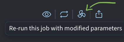
Go back to your analysis overview table and click rerun on your original XDS job. This opens a run-job interface pre-filled to match your previous job.
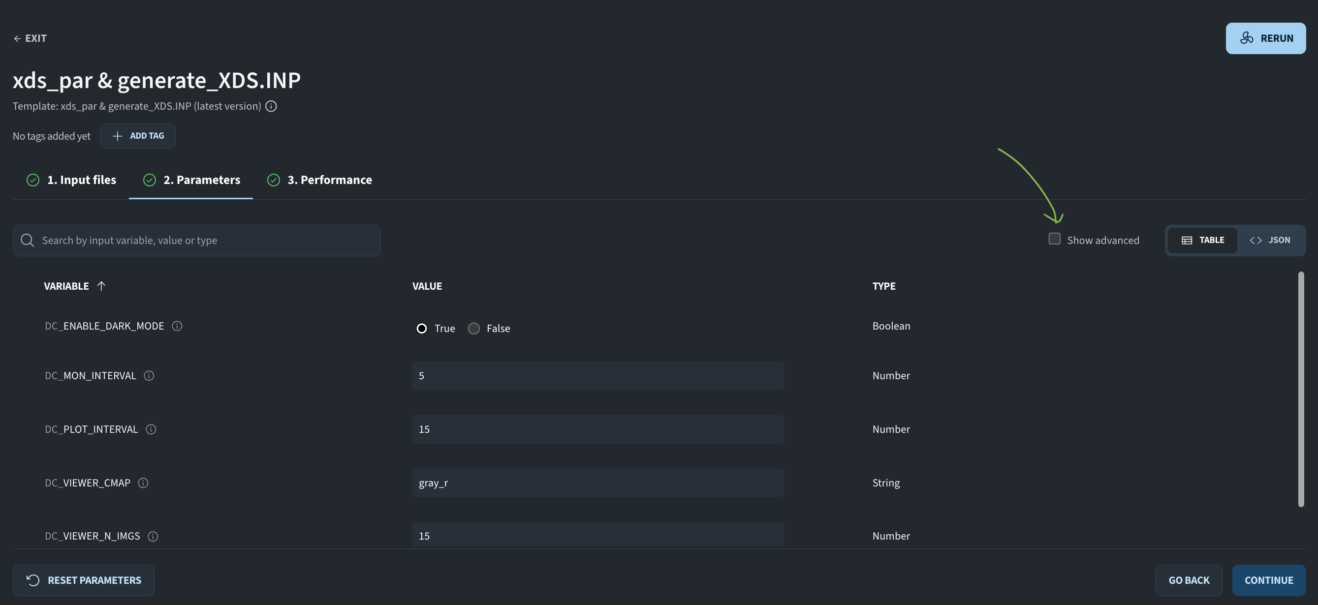
Go to the Parameters tab and click Show advanced to reveal the parameters that override the corresponding keyword in XDS.INP. For example, setting DC_XDS_SPACE_GROUP to 150 changes SPACE_GROUP_NUMBER=0 to SPACE_GROUP_NUMBER=150 in XDS.INP before xds_par runs.
Configure whichever parameters you'd like to experiment with, then click RERUN.
Tag the new job with your dataset name, and optionally with the parameter(s) you're testing.
Inspect the results — what changed as a result of the new parameters?